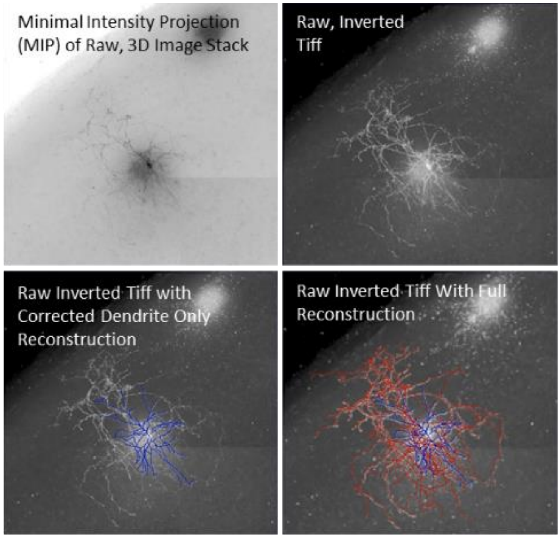
"Reconstuction" is the term of art for morphological analysis that reconstructs the structure of imaged neuron. The above image set illustrates the process.
- The MinIP is the input, the field is bright
- The MinIP inverted for contrast with the blue and red to come
- The reconstructed dendrites overlaid in blue
- The reconstructed axon overlaid in red
Evaluation

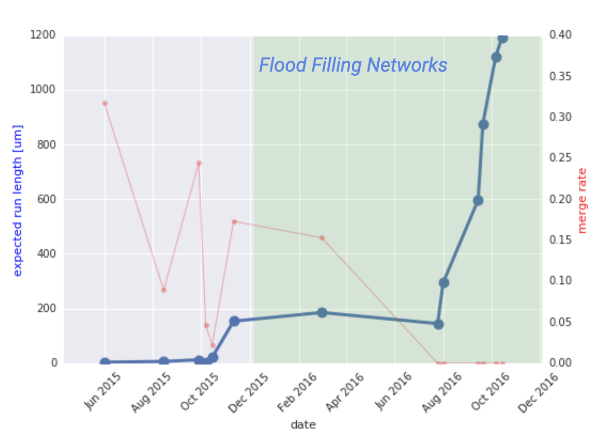
Google uses the "epected run length (ERL)" as a metric of accuracy.
Working with our partners at the Max Planck Institute, we devised a metric we call “expected run length” (ERL) that measures the following: given a random point within a random neuron in a 3d image of a brain, how far can we trace the neuron before making some kind of mistake? This is an example of a mean-time-between-failure metric, except that in this case we measure the amount of space between failures rather than the amount of time. For engineers, the appeal of ERL is that it relates a linear, physical path length to the frequency of individual mistakes that are made by an algorithm, and that it can be computed in a straightforward way.
In contrast to prior approaches, the ERL takes into account the spatial distribution of errors. Previously proposed metrics, such as the total error-free path length (TEFPL) 11,32 and inter-error distance (IED) 11 are defined as simple averages and are thus insensitive to the distribution of lengths of the correctly reconstructed fragments (see Sup. Fig. 2 for an illustration).
Multiple stained cells
In brightfield that is almost always a single neuron. Nonetheless, multiple neurons can be biocytin-stained in the same slice of brain. In such images there is usually little overlap. There is reason to believe that such multi-stained images will be processable via the same algorithms that process single objects. [*]

Banding in the data
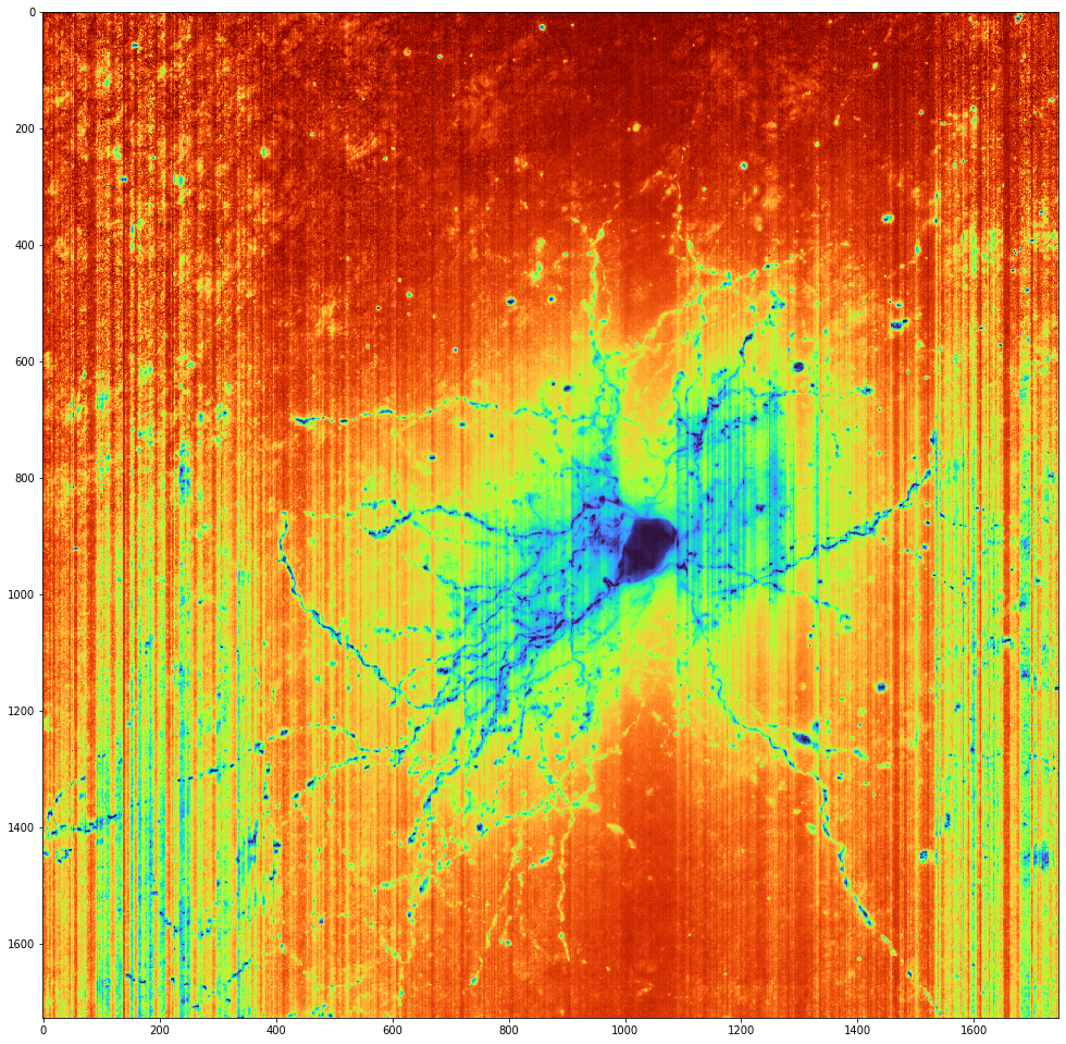
On a semi-local level there is a banding in the data. To see an example, crop in on a random cell's soma. (Here Cell Type DB cell 713686035 is used as an example.) Then using minmax_scale() stretch that subset of the original intensities to the full potential range of 0 -- 255. Finally, colormap to Turbo. The vertical bands alternating yellow and red are some artifact of the input images which the reconstruction algorithms will need to deal with.
import skimage.io
from sklearn.preprocessing import minmax_scale

# Download cell 713686035's stack minimum intensity projection (minip)
!wget --output-document=minip.tif http://reconstrue.com/projects/brightfield_neurons/demo_images/713686035.minip_original.tif
minip_filename = os.path.join(os.getcwd(), 'minip.tif')
minip = PIL.Image.open(minip_filename)

# How much to crop from each side: ((top, bottom), (left, right))
crop_box_for_713686035 = ((2000,2000),(1750,2250))
projection_orig = skimage.io.imread(minip_filename)
minip_cropped = skimage.util.crop(projection_orig, crop_box_for_713686035)
scaled = minmax_scale(minip_cropped) * 255

minip_cropped_pil = PIL.Image.fromarray(scaled)
minip_cropped_pil.show()

References
Other skeletonization methods:
- TEASAR
- seung-lab: Python TEASAR Skeletonization for Sparse Labels
- TEASAR: simple alg, MIT license
- Skeletonize.cpp funkey's C++, MIT
- DeepNeuron: An Open Deep Learning Toolbox for Neuron Tracing
- Vaa3D, Allen Institute 2018
